Symbolic Regression and Genetic Programming

Symbolic regression and genetic programming are nowhere close to being mainstream machine learning techniques. However, they definitely deserve a considerable amount of attention. This post serves as a gentle and informal introduction.

Motivation

Imagine someone asked you to write down the forward pass of a single output neural network without using matrix or sum notation. Huh? To make things simple you would probably think of the most vanilla neural network: Multilayer perceptron with one hidden layer. So in matrix notation, it looks something like

\[\hat{y} =\big(\pmb{\sigma}(\textbf{x} \textbf{W}^{(1)} + \textbf{b}^{(1)})\big)\textbf{W}^{(2)} + b.\]

Ok, in order to drop the matrix notation you would need to decide on the input and hidden layer sizes. Let’s say there are 3 input features and 4 hidden nodes. So your matrices are:

\[\textbf{W}^{(1)} = \begin{pmatrix} w^{(1)}_{11} &w^{(1)}_{12} & w^{(1)}_{13} &w^{(1)}_{14} \\ w^{(1)}_{21}& w^{(1)}_{22} & w^{(1)}_{23}&w^{(1)}_{24} \\ w^{(1)}_{31} &w^{(1)}_{32} & w^{(1)}_{33} & w^{(1)}_{34} \end{pmatrix} , \textbf{b}^{(1)} = \begin{pmatrix} b^{(1)}_1\\ b^{(1)}_2\\ b^{(1)}_3\\ b^{(1)}_4 \end{pmatrix}^{T} , \textbf{W}^{(2)} = \begin{pmatrix} w^{(2)}_1\\ w^{(2)}_2\\ w^{(2)}_3\\ w^{(2)}_4 \end{pmatrix}.\]

Final and the most tedious step is to write everything out without any matrix and sum notation

\[\hat{y} = b + w^{(2)}_{1} \sigma(w^{(1)}_{11}x_1 + w^{(1)}_{21}x_2 + w^{(1)}_{31}x_3 + b^{(1)}_{1} ) \\ + w^{(2)}_{2} \sigma(w^{(1)}_{12}x_1 + w^{(1)}_{22}x_2 + w^{(1)}_{32}x_3 + b^{(1)}_{2} ) \\ + w^{(2)}_3 \sigma(w^{(1)}_{13}x_1 + w^{(1)}_{23}x_2 + w^{(1)}_{33}x_3 + b^{(1)}_{3} ) \\ + w^{(2)}_{4} \sigma(w^{(1)}_{14}x_1 + w^{(1)}_{24}x_2 + w^{(1)}_{34}x_3 + b^{(1)}_{4} ).\\\]

Even though this formulation is extremely impractical it clearly demonstrates one important thing: the prediction is just a result of applying basic mathematical operations on the input features. Specifically, these operations are addition, multiplication and composition. In other words, we combine a bunch of symbolical expressions representing mathematical operations and hope to get the right prediction.

Here is the twist though. With neural networks, one tries to find the optimal values of all the w’s and b’s such that a certain loss function is minimized. However, another idea is to fix all the w’s and b’s and just alter the symbolic expression iteself! Or in other words, change the functional form of the approximator. That is exactly what symbolic regression is about. The altering can naturally have two forms. You can either add new symbolic expressions (mathematical operations) or remove some of the existing ones.

But how?

Unlike in optimizing the weights, with symbolic regression it is not trivial to formulate the problem in a way that gradient descent techniques could be used. However, it is easy to evaluate the performance of a single expression. So how do we come up with this magical expression that achieves a low loss? Enter genetic programming.

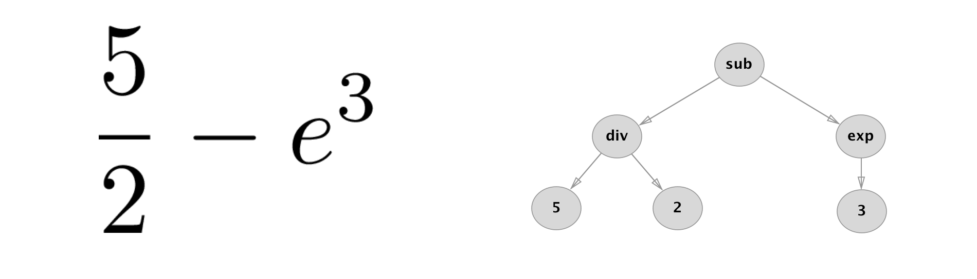
The difference between genetic programming (GP) and the more notorious genetic algorithms (GA) is that GP represents solutions as trees whereas GA as strings. The main reason for using tree representation is the ability to capture the inherent structure of the solution. This is very relevant in our application since each mathematical expression can be represented via a tree. See an example below

Each tree can be assigned a fitness score based on regression metrics like mean squared error or mean absolute error. With GP one also needs to decide on how to perform crossover and mutation. There are a couple of different ways how to do this but let us just describe one simple approach for both of them.

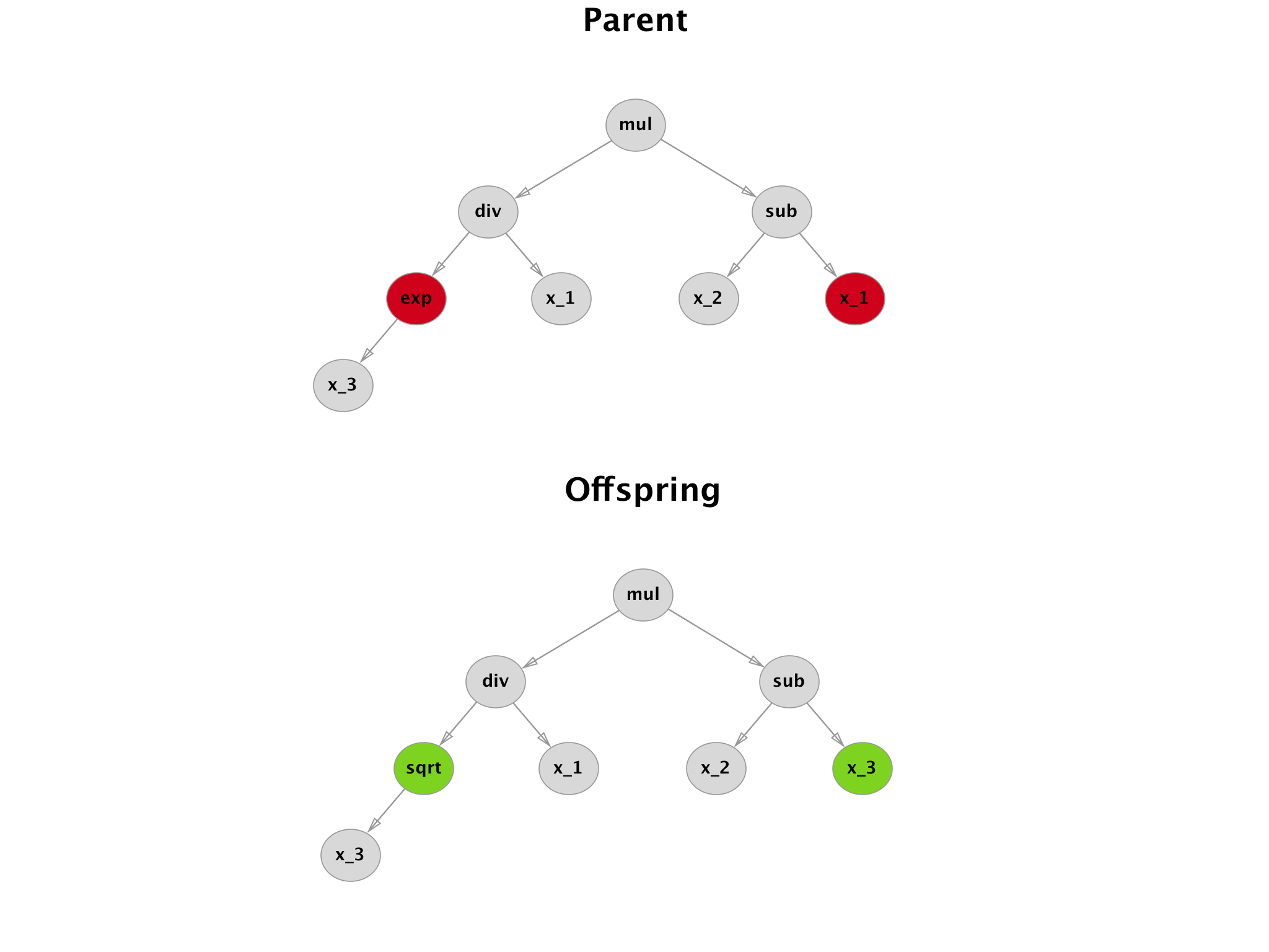
With mutation, the simplest procedure is a so called point mutation. Random nodes of the tree are selected and changed. One needs to be careful about the node type since a node can represent different operations (unary, binary,…).

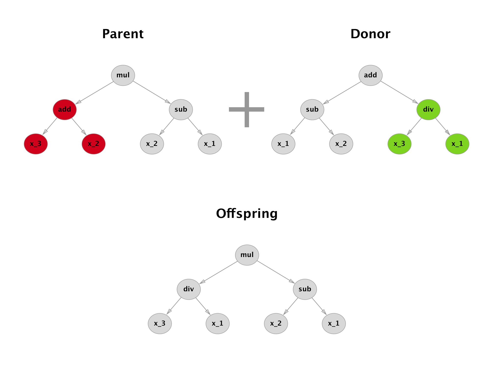
Crossover uses 2 solutions with a high fitness score and tries to combine them. Standard approach is to take a random subtree from the donor and insert it in place of a random subtree of the parent.

gplearn

Of course, you could code everything yourself but there are already open source packages focusing on this topic. The best one I was able to find is called gplearn. It’s biggest pro is the fact that it follows the scikit-learn API (fit and transform/predict methods).

It implements two major algorithms: regression and transformation. With regression, the fitness function is simply a metric like mean squared error or mean absolute erorr. However, transformer creates new features out of the original ones by trying to maximize a fitness function equal to correlation (spearman and pearson).

Once fitted, one can inspect the best solution via the attribute _program. Note that there are multiple hyperparameters that enable customization of all major parts of the evolution. I encourage you to read the official documentation and get familiar with some of them especially if you want to prevent things like overfitting from happening or if you simply look for speedups.

Facebook metrics data set

To illustrate how gplearn works in practice let us take a toy data set called Facebook metrics (link) from the UCI Machine Learning Repository. It has been created based on an undisclosed cosmetics brand Facebook page. See below the attributes of interest.

Attribute name	Possible values
Post Month	1, 2, …, 12
Post Weekday	1, 2, …, 7
Post Hour	1, 2, …, 24
Category	special offer, direct advertisement, inspiration
Type	Link, Photo, Status, Video
Paid	0, 1
Total Interactions	int

The target Total Interactions is a sum of all likes, shares and comments a given post got after it was published. We apply some preprocessing and then train the symbolic regressor. To keep things simple, only the default binary operations are enabled: add, sub, mul, div. The fittest solution after 20 generations is the following.

‘add(add(add(mul(Post Hour, Post Month), sub(Paid_1.0, Category_3)), add(add(mul(Post Hour, Post Weekday), div(mul(Post Hour, Post Month), sub(Category_3, Category_1))), mul(add(Post Weekday, Category_1), add(Type_Photo, Post Month)))), add(sub(Paid_1.0, Category_3), sub(Type_Status, Paid_1.0)))’

Clearly, this textual format is not optimal for visualization. See below a tree representation.

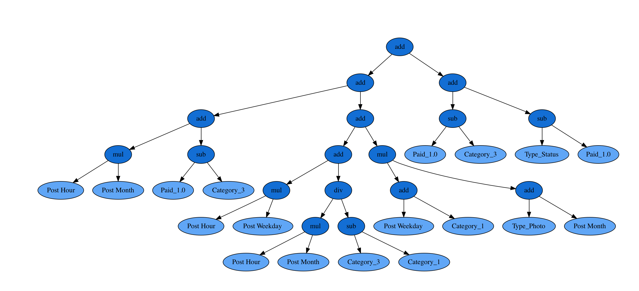
Ehm, so what exactly is this saying? How do I maximize the interactions? Well, it does not really matter. The output of symbolic regression is hard to understand but come on, it is really cool!

If you want to see implementation details and comparison to standard regressors feel free to check the notebook here.

PS

My first encounter with symbolic regression was when I browsed through public kernels on Kaggle (example_1 and example_2). Expecting some elaborate code snippets, I could not help but laugh when I saw these monstrous formulas that managed to get a very decent score in the official leaderboard.

References

1. Koza, John R. “Genetic programming as a means for programming computers by natural selection.” Statistics and computing 4, no. 2 (1994): 87-112
2. (Moro et al., 2016) Moro, S., Rita, P., & Vala, B. (2016). Predicting social media performance metrics and evaluation of the impact on brand building: A data mining approach. Journal of Business Research, 69(9), 3341-3351.
3. gplearn documentation