
Feature Transformers: Hidden Gems
Arguably, the features that enter a supervised learning model are more important than the model itself. With that being said, it is always very difficult to find how to engineer and preprocess features in order for the classifier/regressor to maximize its performance.
There are multiple feature transformation techniques that constitute a standard part of every data scientist’s toolkit. Things like encoding, imputing and scaling are essential. In some cases, it is clear that a certain transformation will improve the performance. A nice example is scaling numerical features before using any kind of gradient descent algorithms. However, in general, there is not a single best approach of how to preprocess and transform features in order to maximize the predictive potential. So what is the right approach? Well, one simply needs to try different techniques and see which one performs the best.
Recently, I have been working with automated hyperparameter search packages—namely auto-sklearn and tpot. They both try to find pipelines that maximize out of sample performance. Not only are they able to do this in a clever way (metalearning using bayesian optimization or genetic algorithms) but also make the usage embarrassingly simple. Surprisingly, the best performing pipelines often include a similar set of transformers and that is exactly the motivation of this post. Buckle up and enjoy the ride ![]() .
.
What is a transformer anyway?
Following the scikit-learn API, we can define a transformer as any subclass of base.BaseEstimator that implements the fit and transform methods.
Naturally, there are dozens of already implemented transfomers that are nicely documented in the official docs. Their real power, however, becomes evident when using Pipelines. Wait, what? A Pipeline (pipeline.Pipeline) is a sequence of transformers that usually ends with a classifier/regressor. It enables the user to logically connect the preprocessing and the machine learning part of the task, avoid leaking information from train to test set and (most importantly) finding optimal hyperparameters over all steps ![]()
![]()
![]() .
.
Old Friends
Before getting too fancy, let us just list the most frequently used transformers:
- Scalers (
StandardScaler,MinMaxScaler,RobustScaler, …) - Univariate Selectors (
SelectKBest,SelectPercentile, … ) - PCA with kernels
- Polynomial features
Are they good enough? Sure, they prove to be useful time and time again for various data sets and should never be discarded. However, there is no reason not to explore further.
Gems
Ok, now we are finally ready to look at 3 different techniques that are not as common as the basic ones. However, they have a tremendous potential to generate great features for the final estimator.
Random Trees Embedding
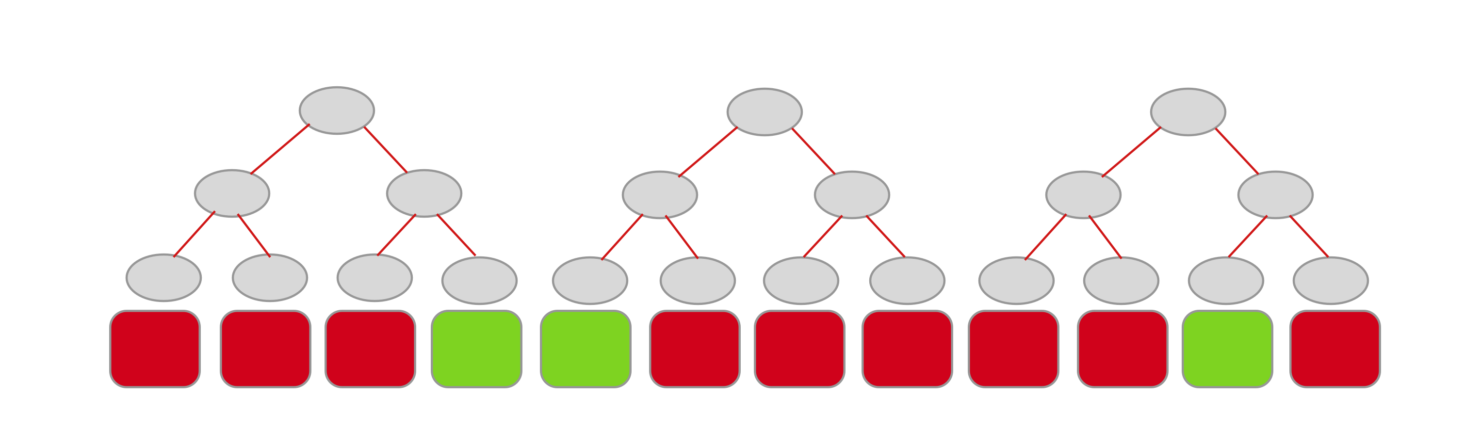
Decision trees/random forests are notorious for being able to capture complicated nonlinear dependecies. One can use this property to generate high-dimensional feature transformation called Random Trees Embedding (RTE). How exactly can this be done? When used as an estimator, a decision tree assigns each sample to a unique leaf node and makes the same predictions within the same nodes. Rather than being focused on the prediction, we can steer our attention to the leaf node itself and use it as a way to encode each sample as a one hot vector. Zeros represent all the leaf nodes our sample did not end up in, whereas the only 1 corresponds to the node our sample arrived at. One can proceed in the same way with an arbitrary number of trees and stack all the implied one hot vectors. This naturally results in a sparse high-dimensional vector. Below is a sketch of this idea for 3 decision trees—green features correspond to a 1, red ones to a 0.
RTE is an unsupervised algorithm that achieves the above by generating totally random trees! The implementation is readily available in scikit-learn under ensemble.RandomTreesEmbedding. Some of the more relevant parameters are:
-
n_estimators— number of trees -
max_leaf_nodes— maximum leaf nodes per tree (the actual number can be lower)
These two parameters allow us to control the dimensionality of transformed features. The dimension will be at most n_estimators * max_leaf_nodes.
Stacking Estimator
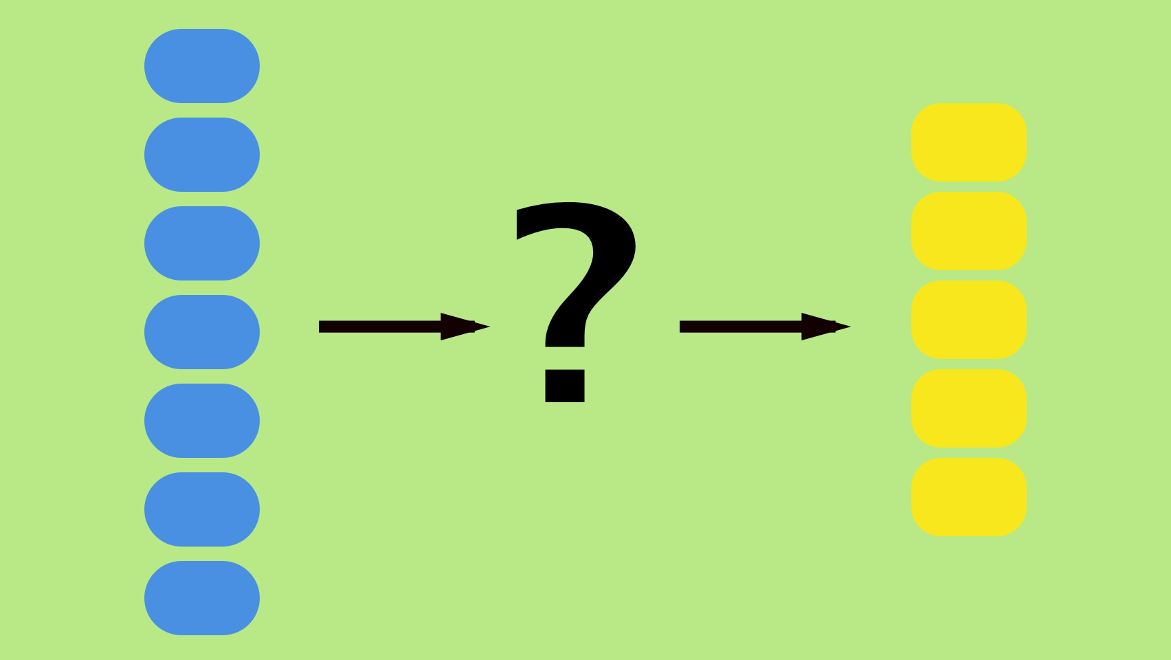
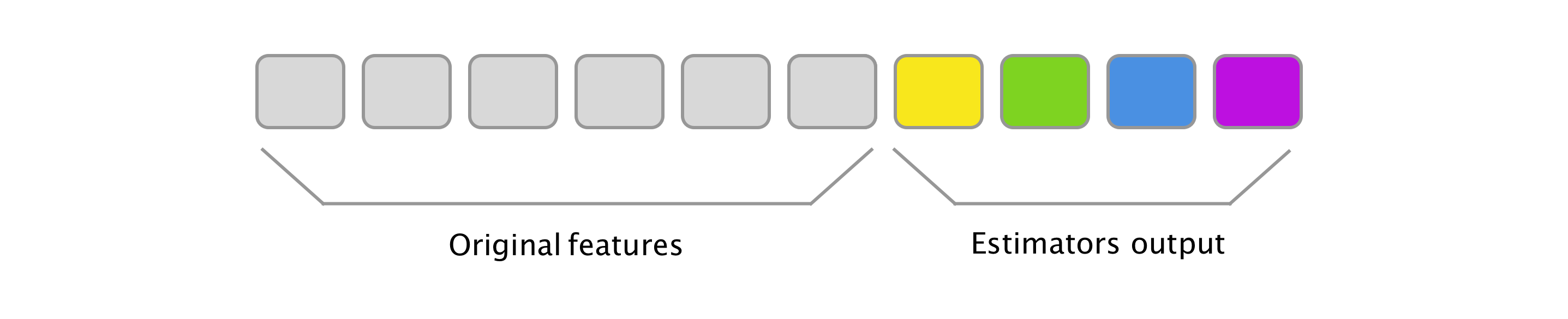
Ensemble learning is a set of broadly used techniques that enable combining different models into one model. The most common techniques are bagging and boosting. However, let us focus on their evil twin—stacking. The goal of Stacking Estimator (SE) is to create meta features from the original ones. Firstly, an estimator is picked that uses original features as inputs and outputs class probabilities (for classifiers) or predictions (for regressors). Applying the estimator to every sample, we can think of the outputs as additional features and combine it with the original feature vector through horizontal stacking. This process can be repeated and different estimators added (input is always the original features). Naturally, one can even nest this process (input is the original features together with output of all previous estimators).
See below a possible mental picture you can assign to stacking in your head (or maybe just see some more elaborate diagrams on www provided in the references ![]() ).
).
Since Stacking Estimator is not a part of scikit-learn, one needs to look somewhere else (mlxtend) or create this transformer himself. A minimal version is shown below.
import numpy as np
from sklearn.base import BaseEstimator, TransformerMixin

class StackingEstimator(BaseEstimator, TransformerMixin):
    """Stacking estimator"""

    def __init__(self, estimator):
        self.estimator = estimator  # instance of sklearn regressor or classifier

    def fit(self, X, y=None, **fit_params):
        self.estimator.fit(X, y, **fit_params)
        return self

    def transform(self, X):
        if hasattr(self.estimator, 'predict_proba'):
            X_transformed = np.hstack((X, self.estimator.predict_proba(X)))
        else:
            X_transformed = np.hstack((X, np.reshape(self.estimator.predict(X), (-1, 1))))

        return X_transformed
Recursive Feature Elimination
In situations where we have too many features it is desirable to have a transformer that is purely feature selecting. That means that the actual transformation consists of dropping a certain number of features while leaving the remaining ones intact.
Recursive feature elimination (RFE) does exactly this through an iterated procedure. Like with many other transformers, scikit-learn has a great implementation of this algorithm under feature_selection.RFE.
Let us briefly describe how things work under the hood. Firstly, one needs to specify the desired dimensionality of transformed features and then the number of features to be dropped during each iteration. The logic underlying feature selection within an iteration is very simple—fit a model that contains coef_ or feature_importances_ and discard the least relevant ones (coef_ closest to zero or lowest feature_importances_).
Virtually any linear model can be used to obtain coef_ but preferably a regularized/sparse models like Ridge, Lasso and Elastic net should be employed. For feature_importances_, tree based algorithms are natural candidates.
The RFE has these three important hyperparameters:
-
estimator: estimator containing eithercoef_orfeature_importances_ -
n_features_to_select: final number/percentage of features we want to arrive at -
step: number/percentage of features to remove at each iteration
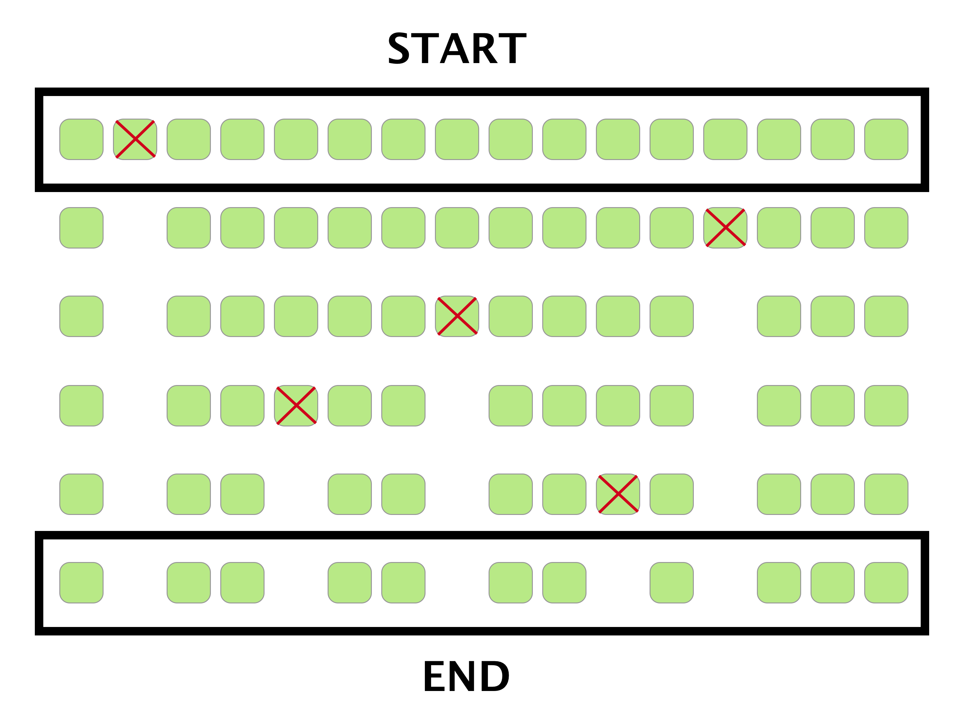
See below an example where n_features = 16, step = 1 and n_features_to_select = 11.
Note that if you do not a priori know what the n_features_to_select should be, consider using a cross-validated version of this algorithm under feature_selection.RFECV.
Conclusion
This post described basic logic behind 3 off-the-shelf transformers. Two of these transformers increase the dimensionality of the feature vector— Random Trees Embedding and Stacking Estimator. The third one, Recursive Feature Elimination, reduces the dimensionality. While SE and RFE are very general and can be applied with success to any problem at hand, RTE is more domain specific.
Naturally, there are dozens of other amazing transformers that were not discussed. Let us at least give some of them a honorable mention — FastICA, Random Kitchen Sinks, Autoencoders, Feature Agglomeration and Manifold Learning.


Leave a Comment