Creating animations with MCMC

Introduction

Markov Chain Monte Carlo (MCMC) is a widely popular technique in Bayesian statistics. It is used for posteriori distribution sampling since the analytical form is very often non-trackable. In this post, however, we are going to use it to generate animations from static images/logos. Incidentally, it might serve as an introduction to MCMC and Rejection sampling. The idea is based on a great open source package imcmc (link) that is built upon PyMC3 (link).

Preliminaries

While MCMC is applicable in any dimension, we are going to focus on 2D distributions. Why? Well, check the below diagram.

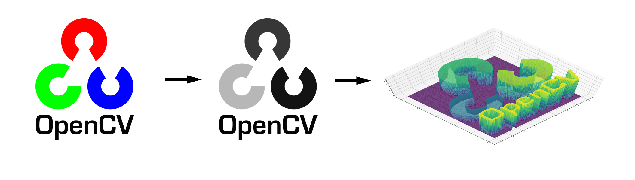
We start with an RGB image (preferably a simple logo), turn it into grayscale and assign each pixel a probability based on intensity. In our case, the darker the pixel the higher the probability. This results in a discrete 2D distribution.

Once we have this distribution we can draw samples (pixels) from it. In general, we look for the following 2 properties:

1. The samples really come from the target distribution
2. The succession of samples and their visualization is aesthetically pleasing

While the 2nd property is always in the eye of the beholder, the 1st one can be achieved by using appropriate sampling algorithms. Specifically, let’s have a closer look at 3 sampling algorithms that are very well suited for the problem at hand: Rejection, Gibbs and Metropolis-Hastings sampling.

Sampling schemes

Rejection sampling

The first method falls into the class of IID (independent and identically distributed) sampling methods. This essentially means that current sample will have no effect on what the next sample is going to be. The algorithm assumes we are able to sample from a so called proposal distribution. Many different proposal distributions can be used but the most common ones are the Uniform (finite support) and the Normal (infinite support) distribution.

To minimize the probability of rejecting samples, it is essential that we select a proposal distribution that is as similar to our target as possible. Also, we want the scaling constant M to be as low as possible. See below (1D) scheme of Rejection sampling.

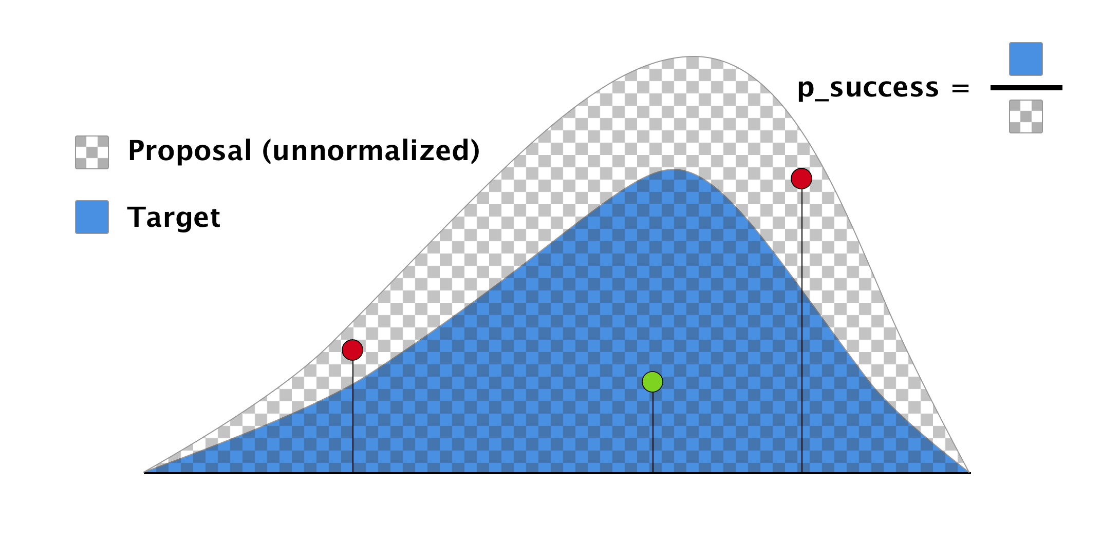
In our setting, we can take a 2D uniform distribution to serve as the proposal.

def rejection_sampling(image, approx_samples):

    image_pdf = image / image.sum()
    pdf_max = image_pdf.max()
    height, width = image_pdf.shape
    p_success = 1 / (height * width * pdf_max)
    actual_samples = min(int(approx_samples / p_success), int(1e8))

    samples_height = np.random.randint(0, high=height, size=actual_samples)
    samples_width = np.random.randint(0, high=width, size=actual_samples)
    samples_uniform = np.random.uniform(0, 1, size=actual_samples)

    result = [(h, w) for (h, w, u) in zip(samples_height, samples_width, samples_uniform) if
                    (image_pdf[h, w] >= pdf_max * u)]

    return result

In lower dimensions, Rejection sampling performs really well. However, with increasing number of dimensions it suffers from the infamous curse of dimensionality. Luckily for us, 2D is not cursed and therefore Rejection sampling is a great choice.

Gibbs sampling

Gibbs sampling falls into the second category of samplers that generate samples via construction of a Markov chain. As a result, these samples are not independent. In fact, they are not even identically distributed until the chain reaches its stationary distribution. For that reason, it is a common practice to discard the first x samples to make sure that the chain “forgot” the initialization (burn-in).

The algorithm itself assumes we are able to draw samples from conditional distributions along every dimension of the target. Whenever we sample from these univariate distributions, we condition on the most recent values of remaining components.

def gibbs_sampling(image, w_start, samples):

    image_pdf = image / image.sum()
    height, width = image_pdf.shape
    result = []
    w_current = w_start

    for _ in range(samples):
        # sample height
        h_given_w = image_pdf[:, w_current] / image_pdf[:, w_current].sum()
        h_current = np.random.choice(np.array(range(height)), size=1, p=h_given_w)[0]

        # sample width
        w_given_h = image_pdf[h_current, :] / image_pdf[h_current, :].sum()
        w_current = np.random.choice(np.array(range(width)), size=1, p=w_given_h)[0]

        result.append((h_current, w_current))

    return result

Metropolis-Hastings sampling

Similarly to Gibbs, Metropolis-Hastings sampling also creates a Markov chain. However, it is more general (Gibbs is a special case) and flexible.

The intuition is the following. Given the current sample, the proposal distribution gives us a suggestion for a new sample. We then assess its eligibility by inspecting how much more (less) likely it is than the current sample and also take into account possible bias the proposal distribution might have towards this sample. Everything combined, we compute the probability $r$ of accepting the new sample and then we let the randomness make the decision.

It goes without saying that the role of the proposal distribution is crucial and will affect the performance and convergence. One of the more common choices is to use the Normal centered at the current state.

Animations

Let’s finally look at some results. For each logo, Rejection and Metropolis-Hastings (using PyMC3) was run and visualization (gifs) was created. The most important hyperparameters:

• burn-in samples: 500
• samples: 10000

Remarks

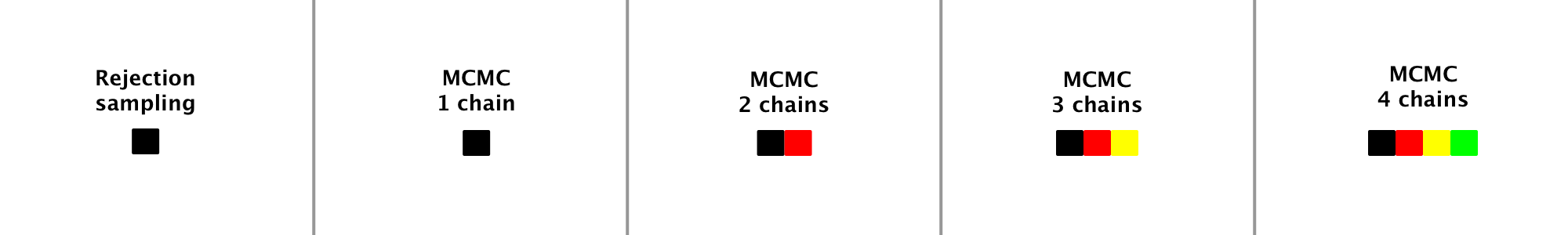
For multimodal distributions Metropolis-Hastings might get stuck in certain regions. This is a very common problem and can be tackled by changing the proposal or sampling more/longer chains. Naturally, we can also venture into the wild and use some other samplers.

If you want to dig deeper and see the source code check this notebook.

References

1. imcmc (https://github.com/ColCarroll/imcmc)
2. PyMC3 (https://github.com/pymc-devs/pymc3)
3. Kevin P. Murphy. 2012. Machine Learning: A Probabilistic Perspective. The MIT Press.